1. Overview
Traditional data mining usually deals with data from a single domain. In the big data era, we face a diversity of datasets from different sources in different domains. These datasets consist of multiple modalities, each of which has a different representation, distribution, scale, and density. How to unlock the power of knowledge from multiple disparate (but potentially connected) datasets is paramount in big data research, essentially distinguishing big data from traditional data mining tasks. This calls for advanced techniques that can fuse the knowledge from various datasets organically in a machine learning and data mining task. These methods focus on knowledge fusion rather than schema mapping and data merging, significantly distinguishing between cross-domain data fusion and traditional data fusion studied in the database community.
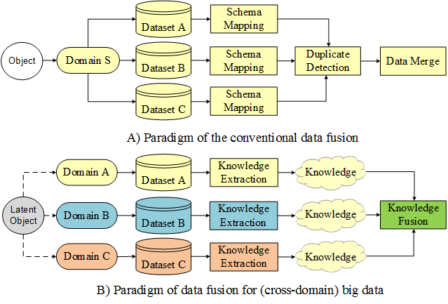
Figure 1. The difference between cross-domain data fusion and conventional data fusion
This tutorial summarizes the data fusion methodologies, classifying them into three categories: stage-based, feature level-based, and semantic meaning-based data fusion methods. The last category of data fusion methods is further divided into four groups: multi-view learning-based, similarity-based, probabilistic dependency-based, and transfer learning-based methods.
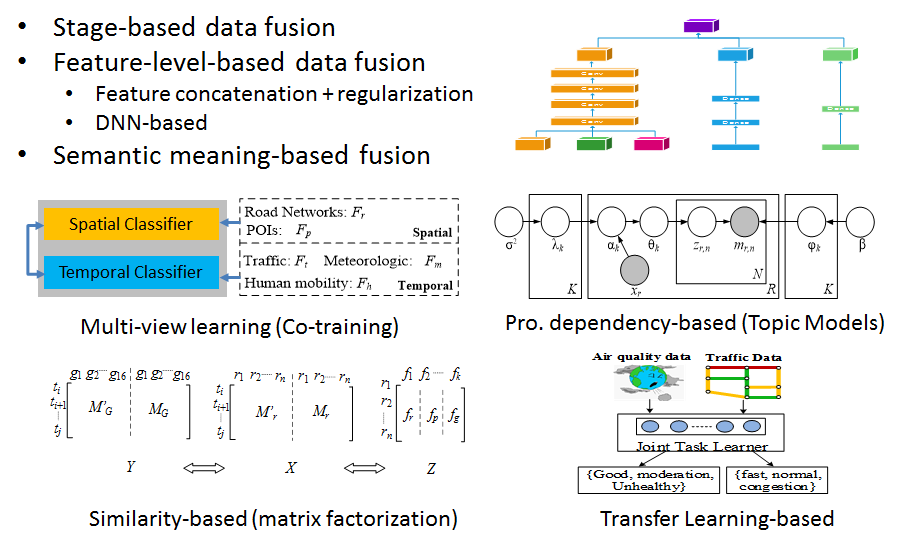
Figure 2 Categories of methods for cross-domain data fusion
This tutorial does not only introduce high-level principles of each category of methods, but also give examples in which these techniques are used to handle real big data problems. In addition, this tutorial positions existing works in a framework, exploring the relationship and difference between different data fusion methods. This tutorial will help a wide range of communities find a solution for data fusion in big data projects.
Yu Zheng. Methodologies for Cross-Domain Data Fusion: An Overview. IEEE Transactions on Big Data, vol. 1, no. 1. 2015.
2. The Stage-Based Data Fusion Methods
This category of methods uses different datasets at the different stages of a data mining task. So, different datasets are loosely coupled, without any requirements on the consistency of their modalities. the stage-based data fusion methods can be a meta-approach used together with other data fusion methods. For example, Yuan et al. [3] first use road network data and taxi trajectories to build a region graph, and then propose a graphical model to fuse the information of POIs and the knowledge of the region graph. In the second stage, a probabilistic-graphical-model-based method is employed in the framework of the stage-based method.
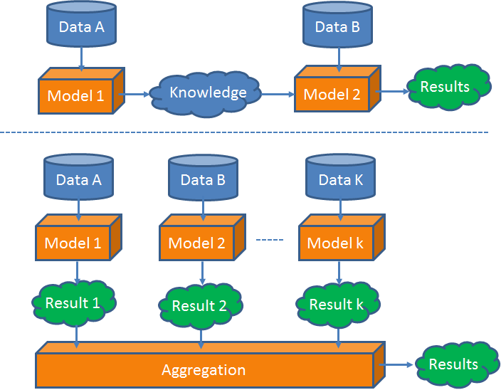
Figure 3. Illustration of the stage-based data fusion
Examples:
As illustrated in Fig. 3 A), Zheng et al. first partition a city into regions by major roads using a map segmen-tation method. The GPS trajectories of taxicabs are then mapped onto the regions to formulate a region graph, as depicted in Fig. 3 B), where a node is a region and an edge denotes the aggregation of commutes (by taxis in this case) between two regions. The region graph actually blends knowledge from the road net-work and taxi trajectories. By analyzing the region graph, a body of research has been carried out to identi-fy the improper design of a road network, detect and diagnose traffic anomalies as well as find urban functional regions.
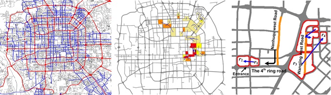
Figure 4. An example of using the stage-based method for data fusion
(Download PPT)
3. The Feature-Level-based Data Fusion
Straightforward methods in this category treat features extracted from different datasets equally, concatenating them sequentially into a feature vector. The feature vector is then used in clustering and classification tasks. As the representation, distribution and scale of different datasets may be very different, quite a few studies have suggested limitations to this kind of fusion. Advanced learning methods in this sub-category suggest adding a sparsity regularization in an objective function to handle the feature redundancy problem. As a result, a machine learning model is likely to assign a weight close to zero to redundant features. More advanced methods have been proposed to learn a unified feature representation from disparate datasets based on DNN.
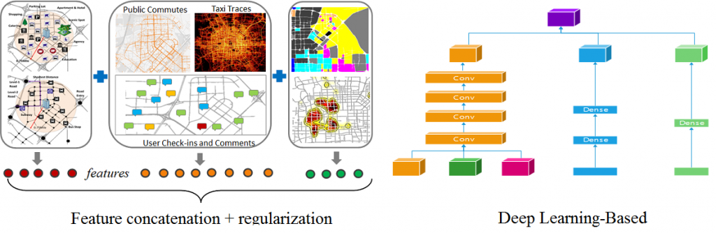
Figure 3. two sub-categories of the feature-level-based data fusion
(Download PPT)
4. The Semantic Meaning-Based Data Fusion
Feature-based data fusion methods do not care about the meaning of each feature, regarding a feature solely as a real-valued number or a categorical value. Unlike feature-based fusion, semantic meaning-based methods understand the insight of each dataset and relations between features across different datasets. We know what each dataset stands for, why different datasets can be fused, and how they reinforce between one another. In addition, the process of data fusion carries a semantic meaning (and insights) derived from the ways that people think of a problem with the help of multiple datasets. Thus, they are interpretable and meaningful. This section introduces four groups of se-mantic meaning-based data fusion methods: multi-view-based, similarity-based, probabilistic dependency-based, and transfer-learning-based methods.
4.1 The Multi-view Based Data Fusion Methods
Different datasets or different feature subsets about an object can be regarded as different views on the object. For example, a person can be identified by the information obtained from multiple sources, such as face, fingerprint, or signature. An image can be represented by different feature sets like color or texture features. As these datasets describe the same object, there is a latent consensus among them. On the other hand, these datasets are complementary to each other, containing knowledge that other views do not have. As a result, combining multiple views can describe an object comprehensively and accurately. The multi-view learning algorithms can be classified into three groups: 1) co-training, 2) multiple kernel learning, and 3) subspace learning. Notably, co-training style algorithms train alternately to maximize the mutual agreement on two distinct views of the data. Multiple kernel learning algorithms exploit kernels that naturally correspond to different views and combine kernels either linearly or non-linearly to improve learning. Subspace learning algorithms aim to obtain a latent subspace shared by multiple views, assuming that the input views are generated from this latent subspace.
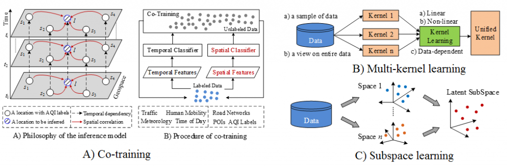
Figure 4. Multi-view learning
(Download PPT)
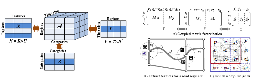
4.2 Similarity-Based Data Fusion Methods
Similarity lies between different objects. If we know two objects (X, Y) are similar in terms of some metric, the information of X can be leveraged by Y when Y is lack of data. When X and Y have multiple datasets respectively, we are can learn multiple similarities between the two objects, each of which is calculated based on a pair of corresponding datasets. These similarities can mutu-ally reinforce each other, consolidating the correlation between two objects collectively. The latter enhances each individual similarity in turn. For example, the similarity learned from a dense dataset can reinforce those derived from other sparse datasets, thus helping fill in the missing values of the latter. From another perspective, we can say we are more likely to accurately estimate the similarity between two objects by combining multiple datasets of them. As a result, different datasets can be blended together based on similarities. Coupled matrix factorization and manifold alignment are two types of representative methods in this category.
(Download PPT)
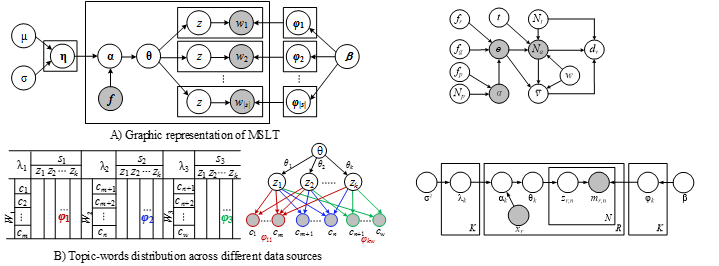
4.3 Probabilistic Dependency-Based Data Fusion Methods
A probabilistic graphical model is a probabilistic model for which a graph expresses the conditional depend-ence structure between random variables. Generally, it uses a graph-based representation as the foundation for encoding a complete distribution over a multi-dimensional space. The graph can be regarded as a compact or factorized representation of a set of independences that hold in the specific distribution. Two branches of graphical representations of distributions are commonly used, namely, Bayesian Networks and Markov Networks (also called Markov Random Field). Both families encompass the properties of factorization and independences, but they differ in the set of independences they can encode and the factorization of the distribution that they induce.
(Download PPT)
4.4 Transfer Learning-Based Data Fusion Methods
A major assumption in many machine learning and data mining algorithms is that the training and future data must be in the same feature space and have the same distribution. However, in many real-world applications, this assumption may not hold. For example, we sometimes have a classification task in one domain of interest, but we only have sufficient training data in an-other domain of interest, where the latter data may be in a different feature space or follow a different data distribution. Different from semi-supervised learning, which assumes that the distributions of the labeled and unlabeled data are the same, transfer learning, in contrast, allows the domains, tasks, and distributions used in training and testing to be different.
In the real world, we observe many examples of transfer learning. For instance, learning to recognize tables may help recognize chairs. Learning riding a bike may help riding a moto-cycle. Such examples are also widely witnessed in the digital world. For instance, by analyzing a user’s transaction records in Amazon, we can diagnose their interests, which may be transferred into another application of travel recommendation. The knowledge learned from one city’s traffic data may be transferred to another city.
![]()
(Download PPT)
People

Yu Zheng
Vice President and Chief Data Scientist, JD Technology Group